In Microsoft Excel, large amount of data is handled by the Pivot table however not many people know that it is a powerful analytical tool for the managers. Before diving into the knowledge base, it is important to know the uses.

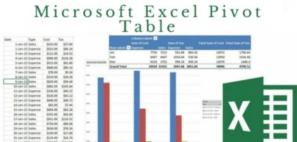
Pivot table is used for summarizing the data reports in a readable format. In addition, the information is summarized into categories and subcategories. People can easily filter and sort out the data into different subsets. By dividing the information, one can spot the trends that might help in taking decision in the near future.

Users are able to create sub totals that are quite useful for business purposes. For instance, Excel Pivot Table assists in summing up the sales information according to the region. In such a case, managers can find the location where the revenues are not meeting expectations. As an entrepreneur, you can also rotate rows and columns to view summaries in different format. There are numerous summing up functions in excel that are used to deliver effective presentations.

Creating Pivot Table:

Microsoft Excel Training suggests that creating pivot table is an absolute breeze and involves few steps as the modern version of the application is extremely fast.

Step 1: Organize The Data Into Rows And Columns

The first step is to organize the data into rows and columns and thereafter it is vital to transform the data range into excel table. In order to accomplish the task, you should click on the insert tab and invoke the table link.
If the source data is excel file, you can reap lots of benefits. The data range can be extended according to the requirements and specifications of the users. In fact, table can be expanded or contracted in real time situation.
Users can add meaningful headings to the columns so that they can be turned into the field’s name.
One should also ensure that the source table is devoid of rows and columns.
In order to name the data source, click on the design tab and enter the table name into the field located in the upper right corner of the worksheet.

Step 2: Select The Source In The Data Table

It is vital to select the source in the data table by choosing all the cells containing the vital information. In addition, people should click on insert tab and invoke the table group menu. Thereafter, click the Pivot table link located beneath the above mentioned link.

It would open the Create Pivot table window right on the screen. Inside the table range field, the whole range of cells in highlighted in the mix. One should also select the target location for the excel pivot table. The new worksheet link would create the table inside the new worksheet right from the top left corner of the sheet. Inside the location box, it is vital to click the collapse Dialog button to identify the first cell for positioning the pivot.

After the process is complete, you need to click on the Ok button in the target location. The pivot table is to be created in a separate worksheet to prevent the cluttering of information. In case, the data is being created from another work sheet incorporate the same by using the inbuilt syntax. As an alternative option, you can always click on the collapse dialog button by selecting range of cells from another worksheet.

In Guide to Microsoft Excel, you can always click on the insert tab and open the charts group. Under the menu, locate the Pivot chart button and invoke the Pivot chart or Pivot table. In other versions, one may find the same under the button.

Step3: Creating The Layout For The Data

One of the most popular aspects of the Pivot table is that it has a user friendly interface. The area in which the fields of pivot table are to be placed is also called the PivotTable Fieldslist. It is situated in the right hand side of the worksheet to segregate the header and body sections.

Field section comprises of the names of the fields that can be placed into the pivot table. Field names are in fact the column names of the pivot table. Lay out section comprises of the report filter section along with the Column labels and Row labels. The fields could be arranged in a definite format in the pivot table.

Once the modifications are made into the PivotTablefields list, they are immediately reflected in the table on the sheet. Hence, you can get the results instantly to facilitate decision making process.

Step 4: Remove Field From The Pivot Table

In order to remove field from the pivot table, you should uncheck the check box nest located in the field section of the PivotTable pane. You can also right click on the field located in the pivot table and invoke the Remove Field_name option.

Step 5: Arranging The Fields In The Layout Section Can Be Performed In Namely Three Ways

It is important to drag and drop fields between the 4 areas of the layout section by deploying the mouse. You can either click or hold the field name inside the field section of the pivot table. Once the process is completed, drag the same into the layout section to the main area.
Thereafter, right click on the field name and also locate the area where it is to be added. After accessing the layout menu, you should select the optin available for the field. It is a short and simple process that even a layman can perform.

Step 6: Select The Suitable Function To Pass Values

Generally Excel Formulas includes sum function inside the sheet by default however there are many options available for the users. In case, numeric data populates the cell, count function is activated.

In order to get customized summary function, click on the value field and select the summarize field value by option in the context menu. Some of the alternatives include average, Max and Min. To get advanced alternatives, click on the more options and summarize the data according to the specifications. One can also access the full list of functions to get the best report.